
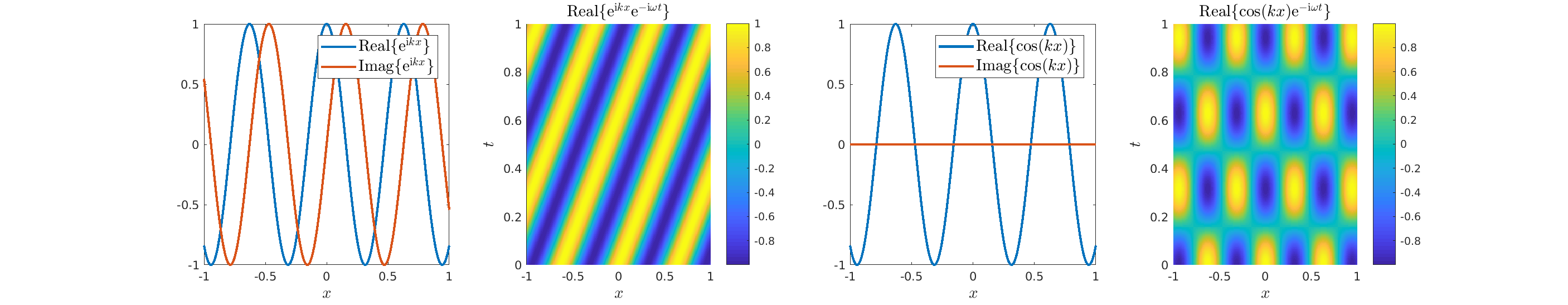
Solutions of the Helmholtz equation in 1 dimension: travelling wave \(u(x)=\mathrm e^{\mathrm ikx}\) and standing wave \(u(x)=\cos(kx)=\frac{\mathrm e^{\mathrm ikx}+\mathrm e^{-\mathrm ikx}}2\), and their evolution in time \(U(x,t)=\Re\{u(x) \mathrm e^{-\mathrm ikt}\}\).
Motion of the particles in a fluid subject to an acoustic plane wave \(U(\mathbf{x},t)=\cos(k(x_1-ct))\).
Each particle oscillates harmonically back and forth, but remains in a small region.
The blue line represents the acoustic pressure (or the density).
Time-harmonic elastic plane waves in a solid:
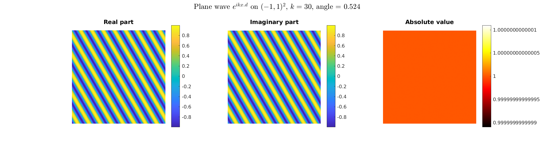
travelling P-wave \(\mathbf d \mathrm e^{\mathrm ik\mathbf x\cdot\mathbf d}\),
travelling S-wave \(\mathbf A \mathrm e^{\mathrm ik\mathbf x\cdot\mathbf d}\),
stationary P-wave \(\mathbf d \sin(k\mathbf x\cdot\mathbf d)\),
stationary S-wave \(\mathbf A \sin(k\mathbf x\cdot\mathbf d)\)
(\(\mathbf d\cdot\mathbf A=0\)).
P-wave = pressure wave = primary wave = longitudinal wave.
S-wave = shear wave = secondary wave = transverse wave.
Travelling (transverse) S-wave \(\mathbf A\mathrm e^{\mathrm i k \mathbf x\cdot\mathbf d}\):
linear polarisation \((0,0,1)^\top\mathrm e^{\mathrm i kx_2}\),
circular polarisation \((\mathrm i,0,1)^\top\mathrm e^{\mathrm i kx_2}\).
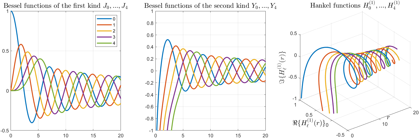
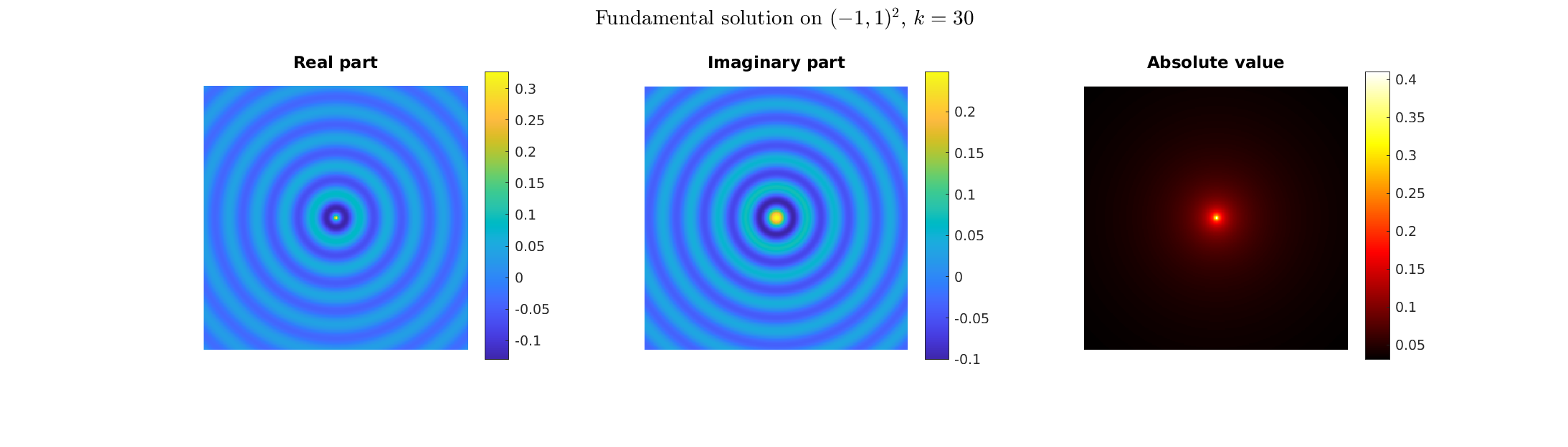
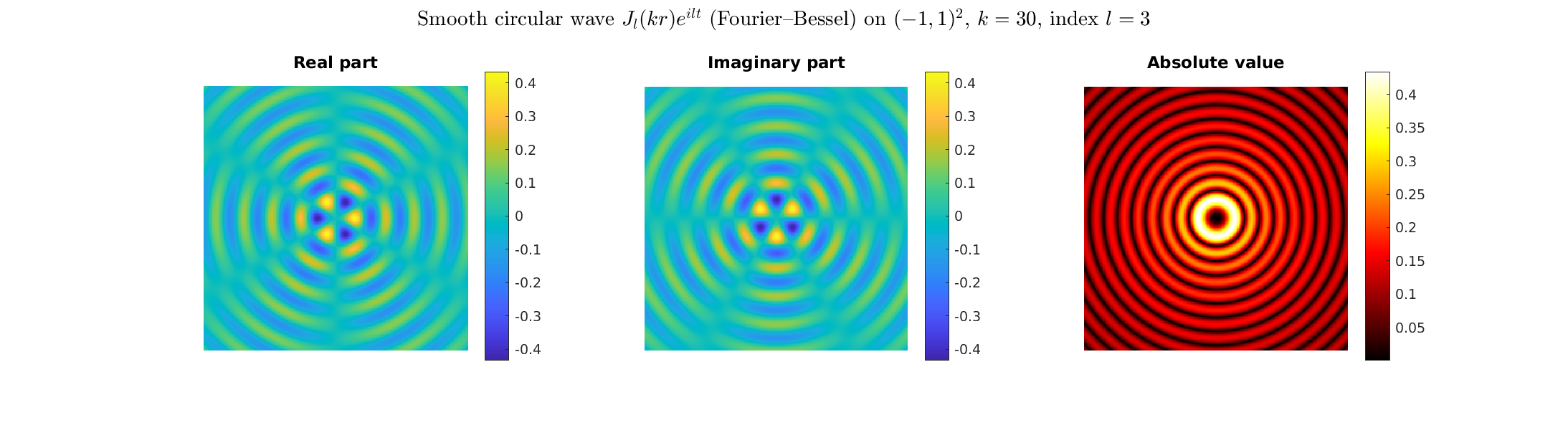
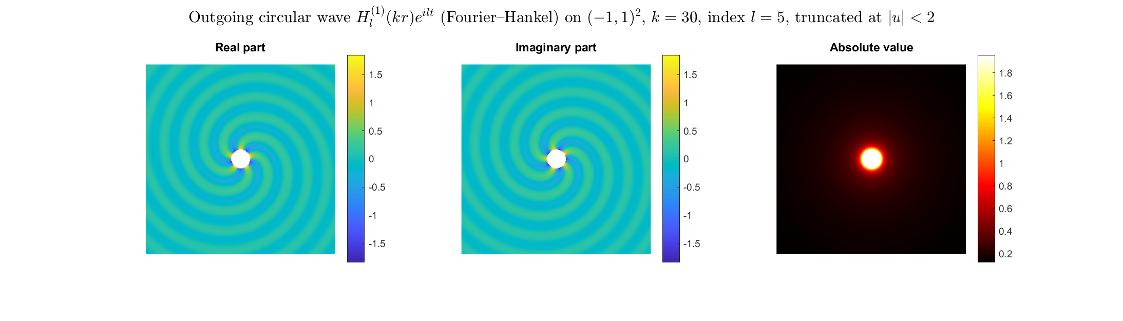
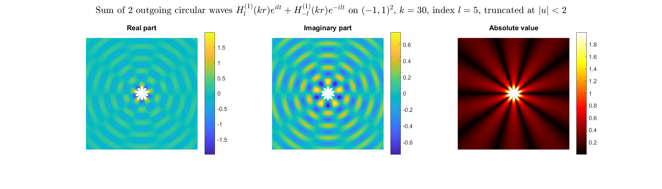
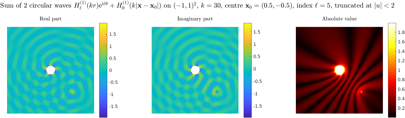
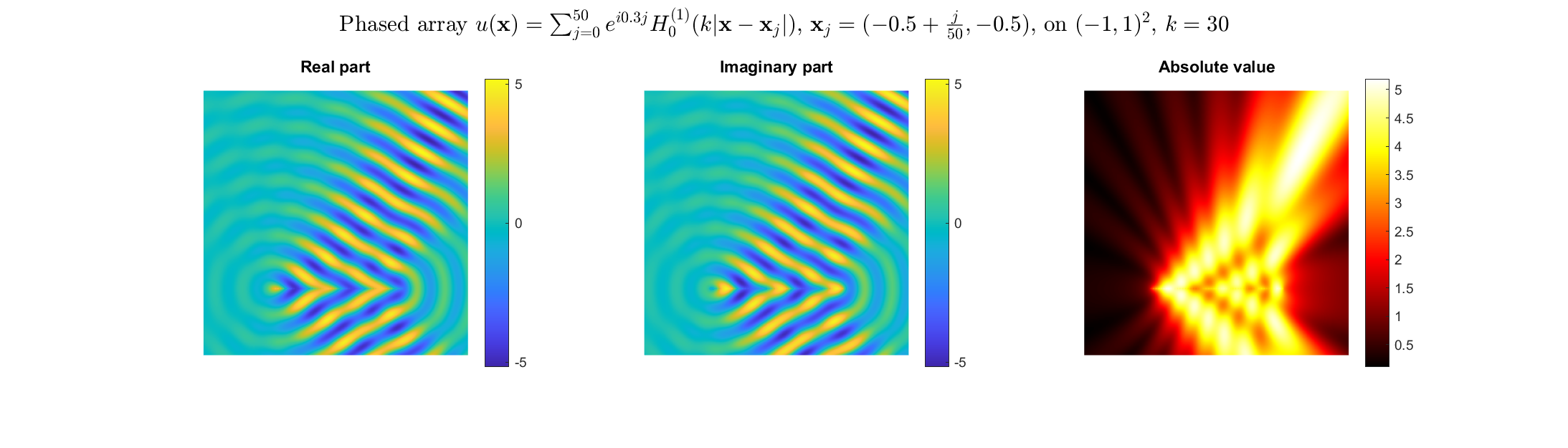
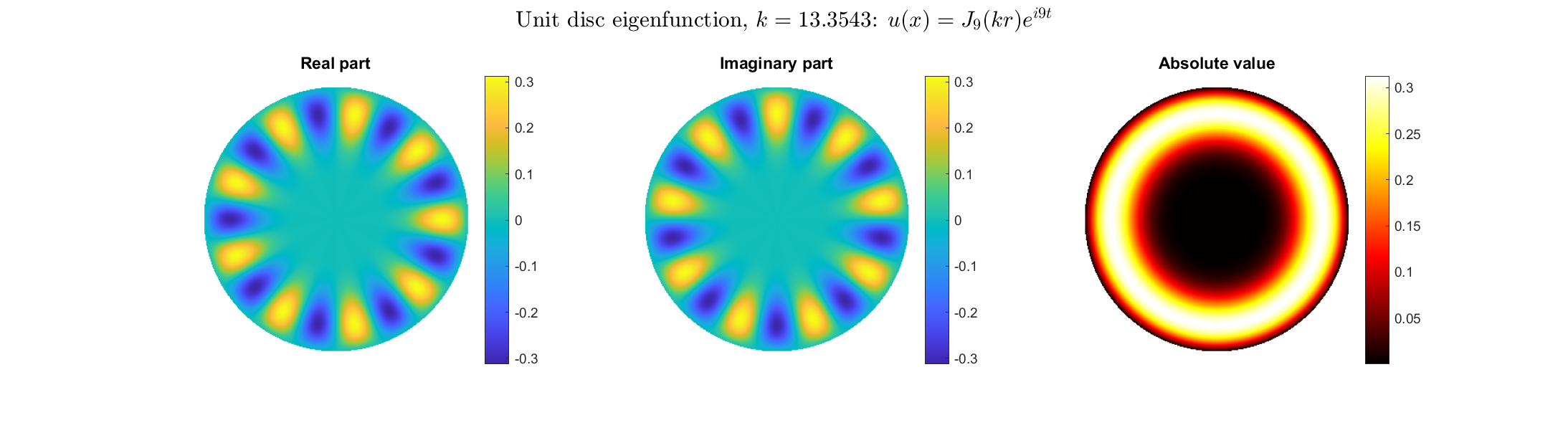
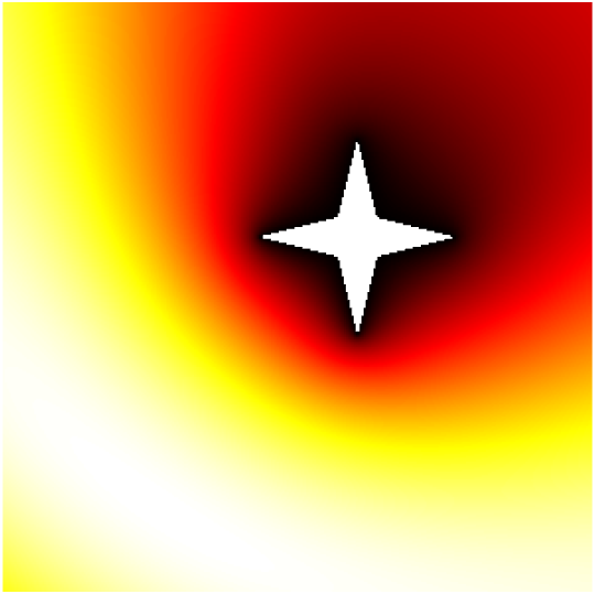
Bessel and Hankel functions.
|
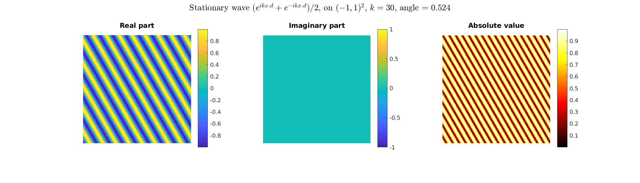
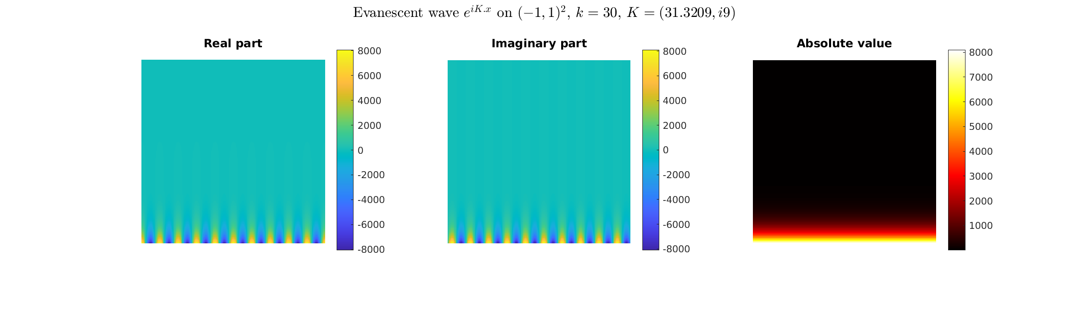
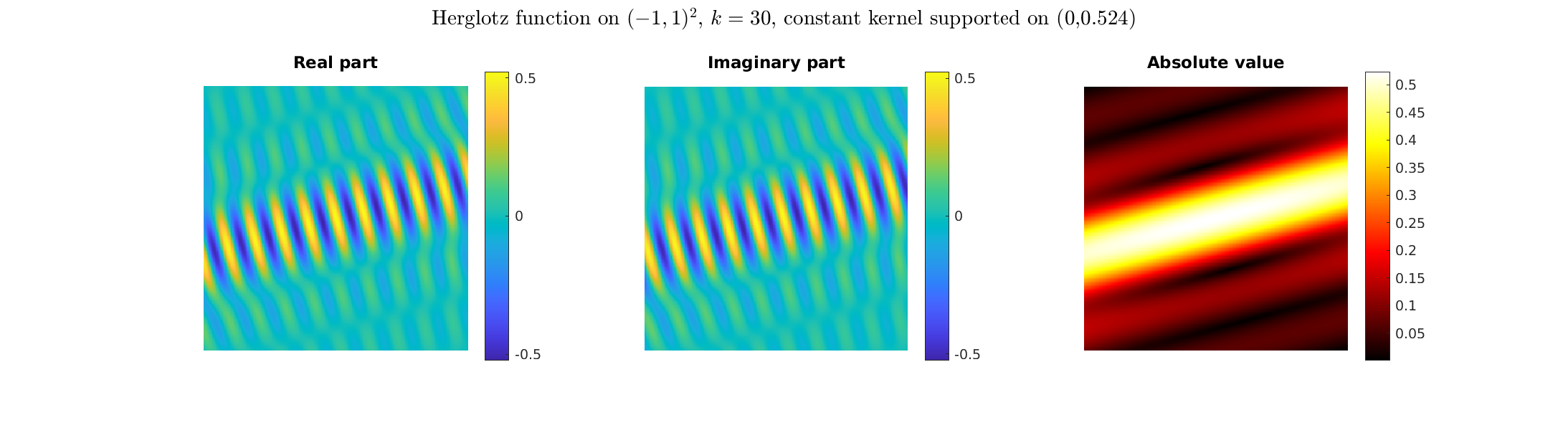
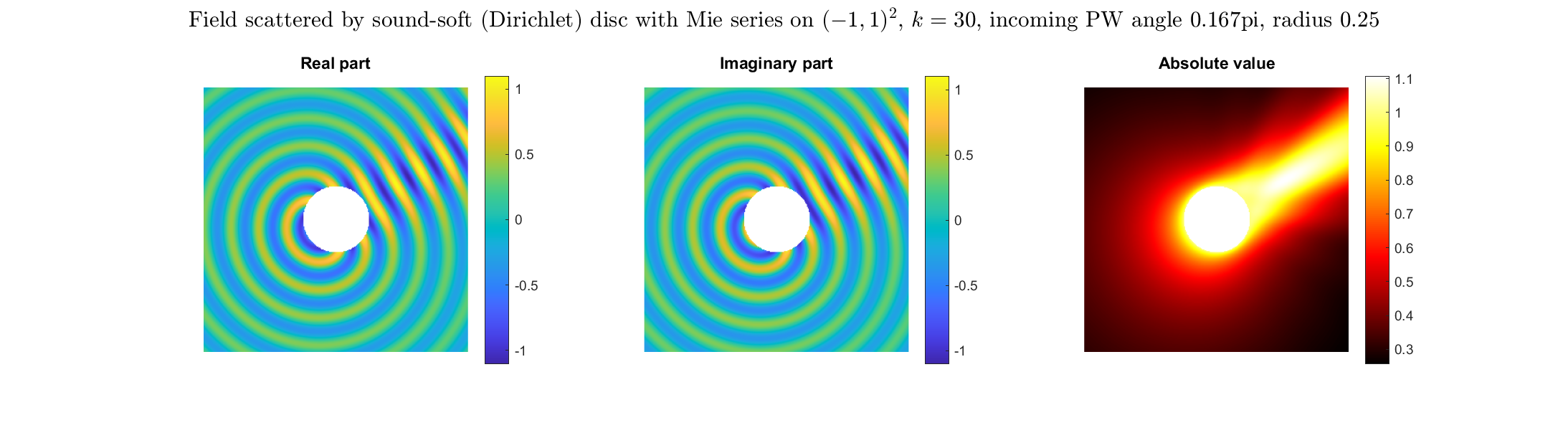
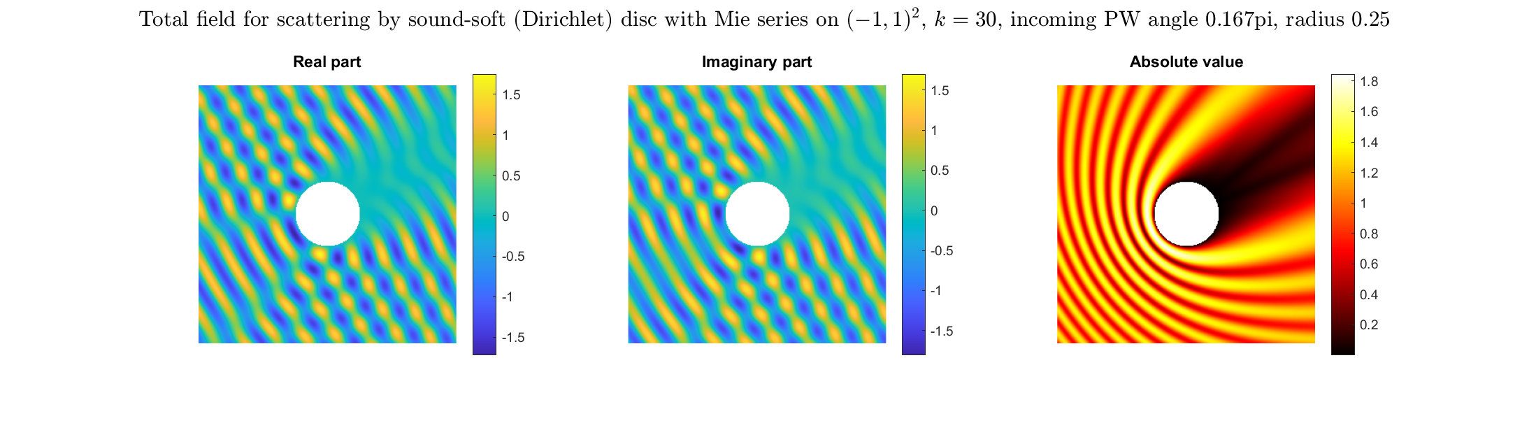
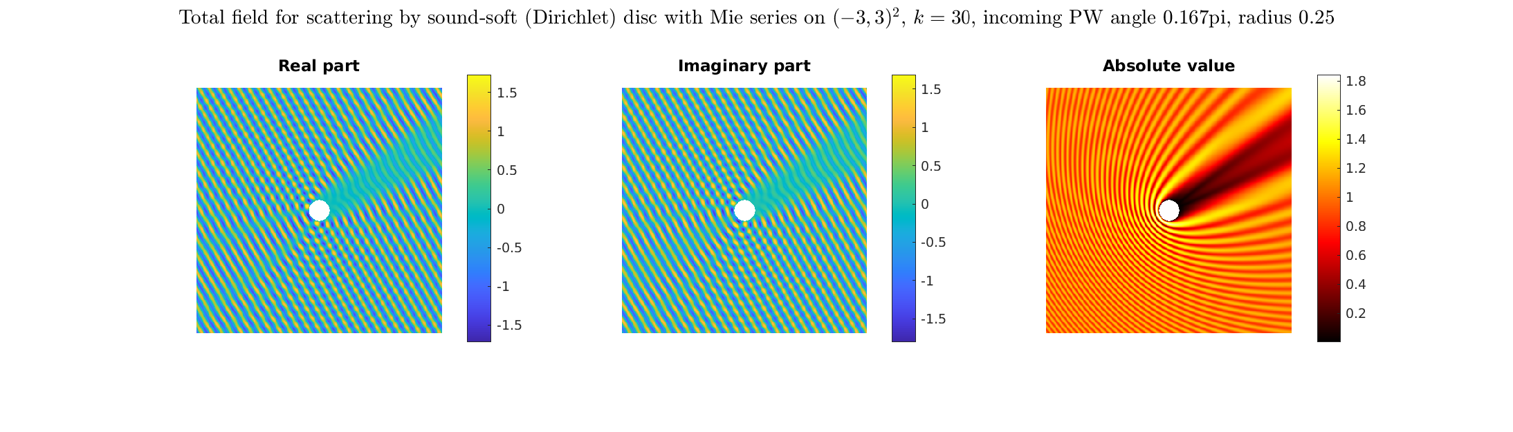
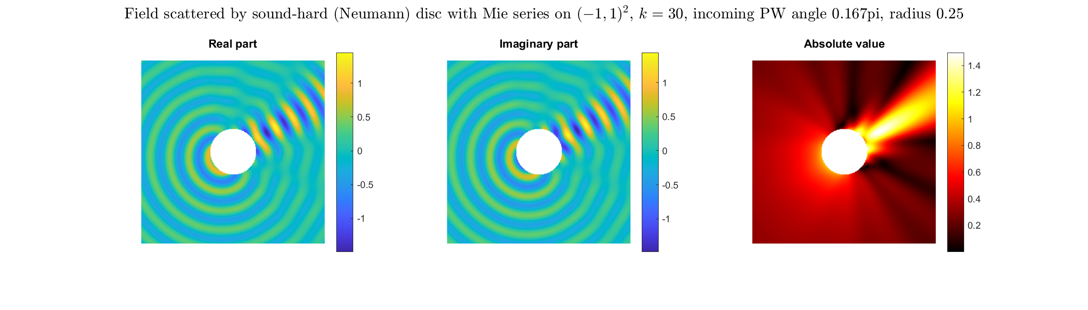
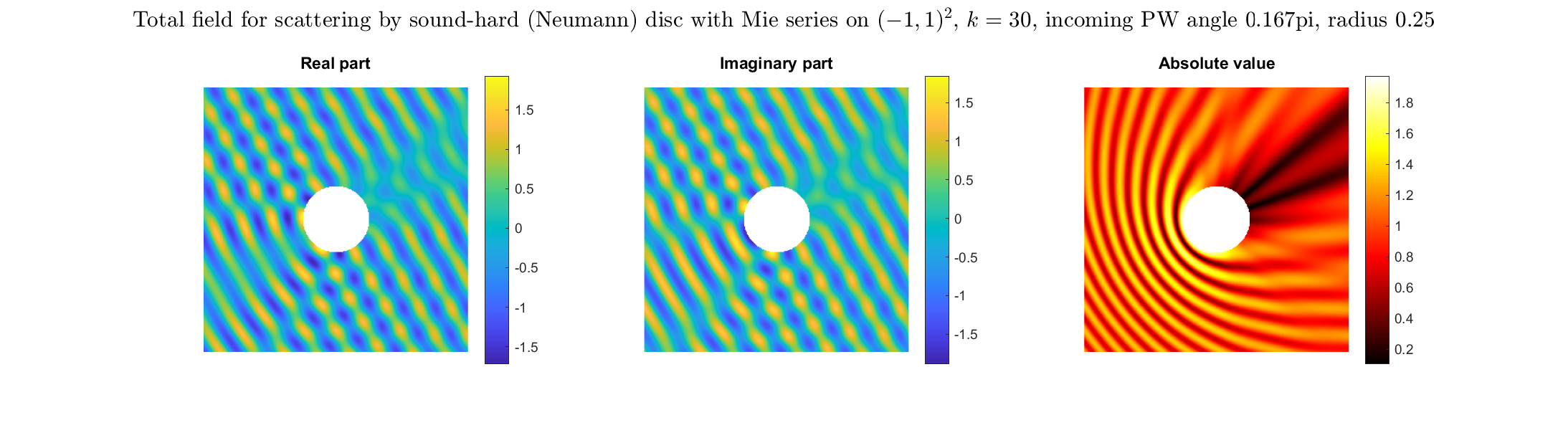
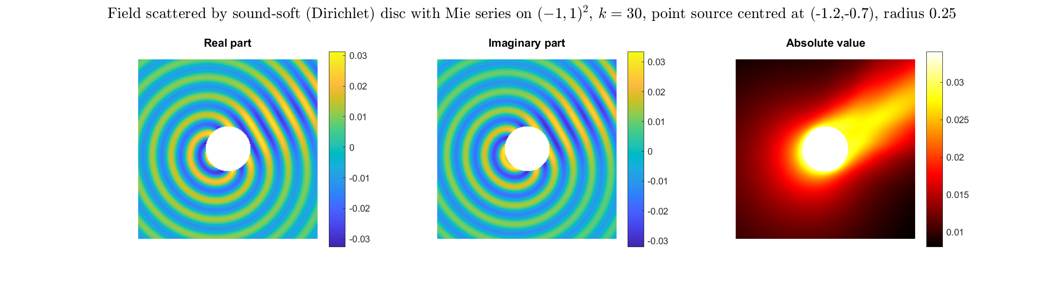
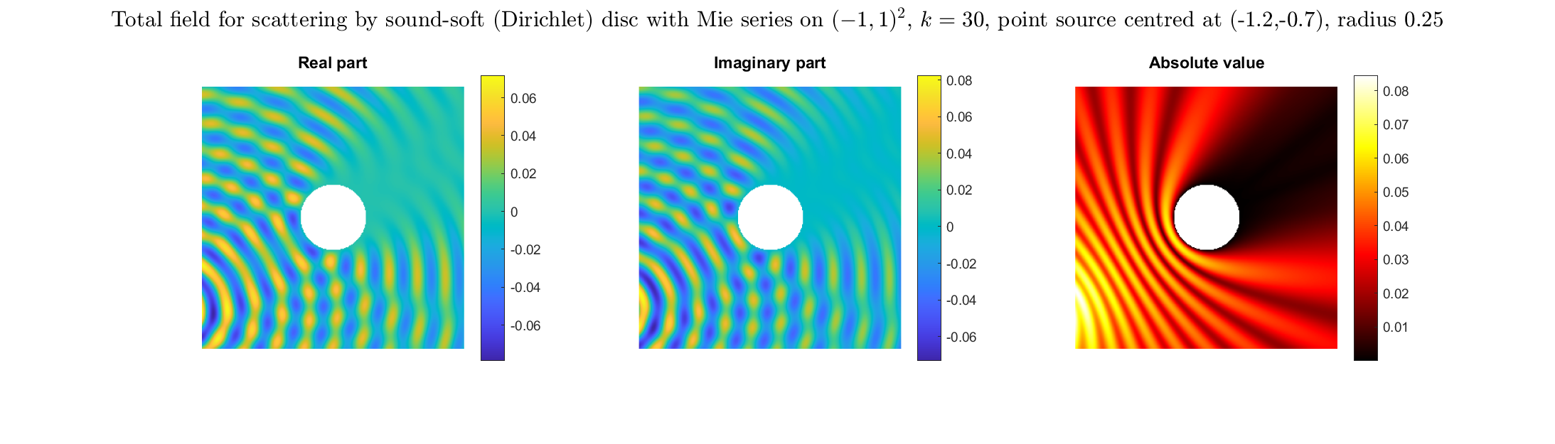
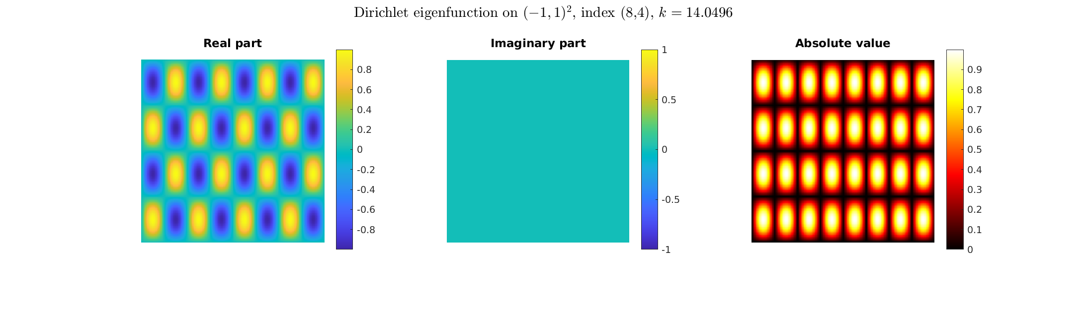
Special solutions of the Helmholtz equation in 2 dimensions: real and imaginary parts, magnitude and time evolution.
|
|
|
|
|
|
|
|
|
|
|
|
|
|
|
|
|
|
|
|
|
|
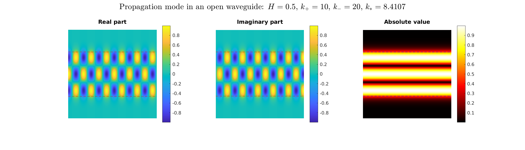
Transmission problems: solutions of the Helmholtz equation with piecewise-constant wavenumber
|
|
|
|
|
|
|
|
|
|
\(n=1/3\)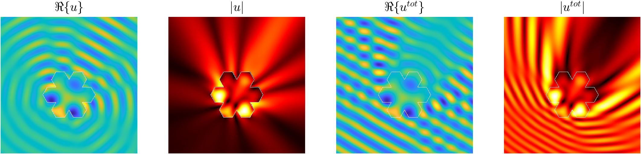
|
\(n=1/2\)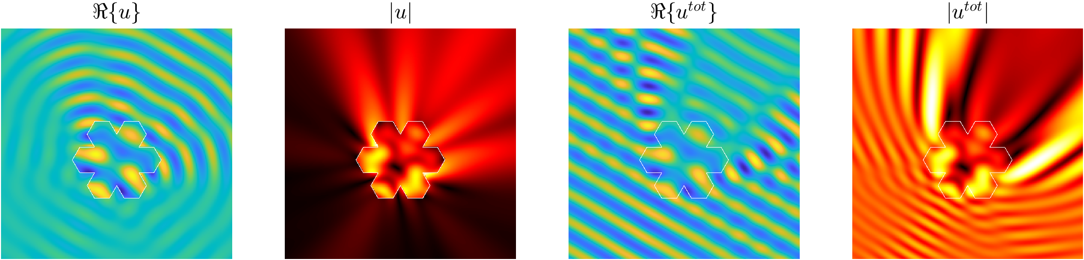

|
\(n=2\)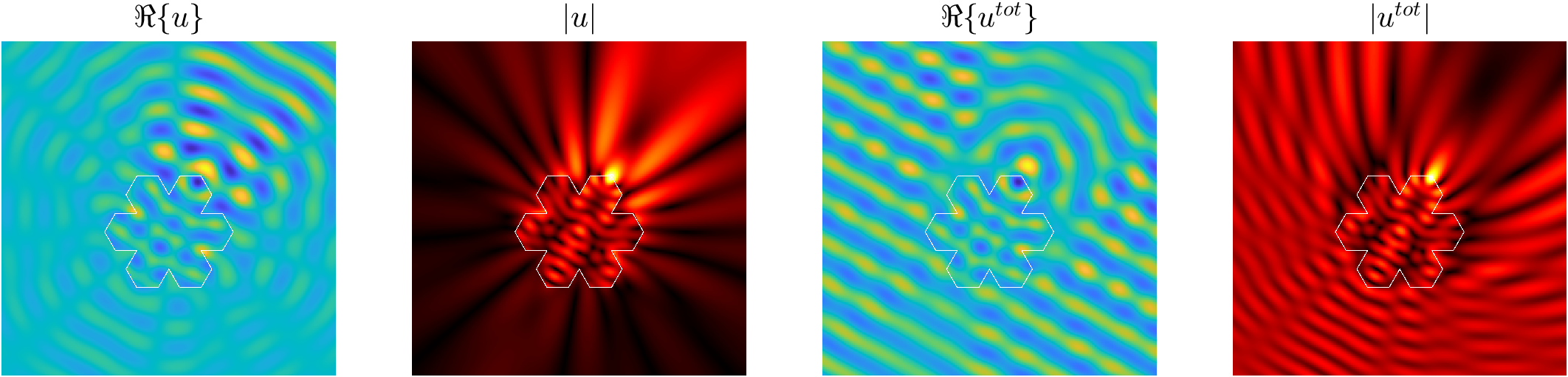
|
\(n=3\)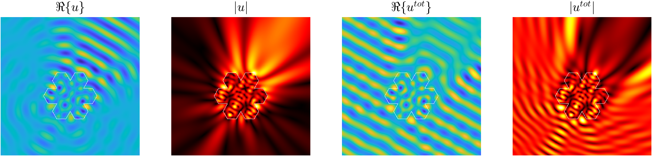
|
\(n=4\)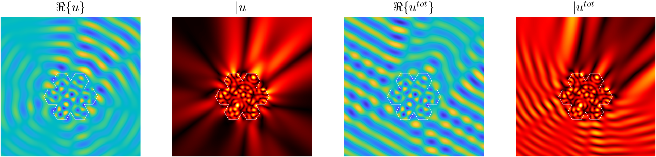
|
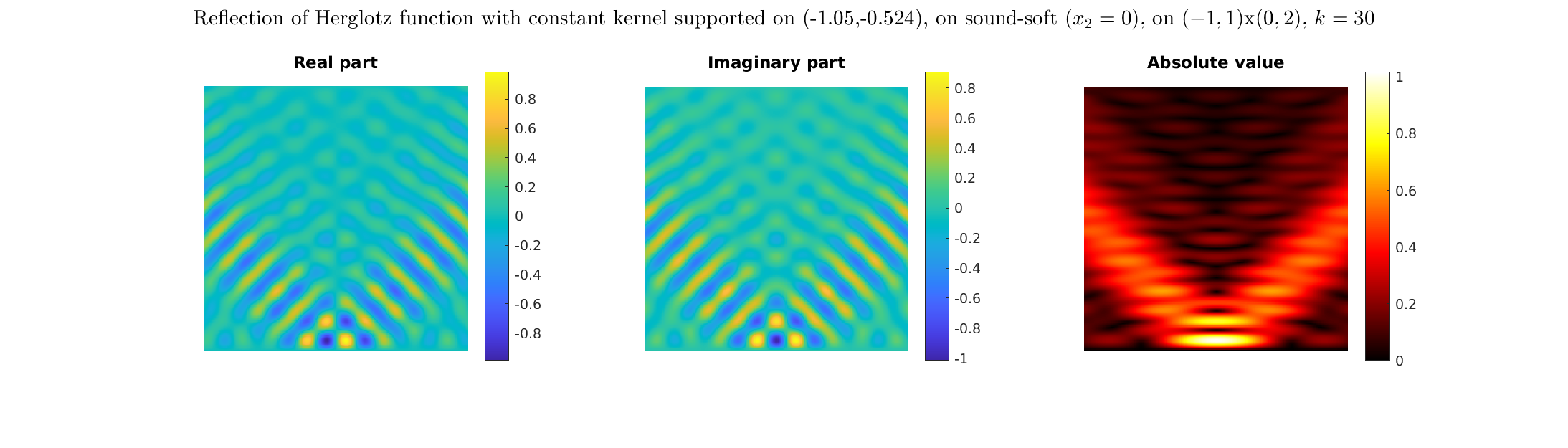
Plane wave of direction \((\frac{\sqrt3}2,-\frac12)\) reflected by the horizontal line \(\{x_2=0\}\).
On the lower side of the square we have imposed sound-soft (\(u=0\)), sound-hard (\(\partial_n u=0\))
and impedance (\(\partial_n u-\mathrm ik\vartheta u=0\), \(\vartheta=1\)) boundary conditions, respectively.
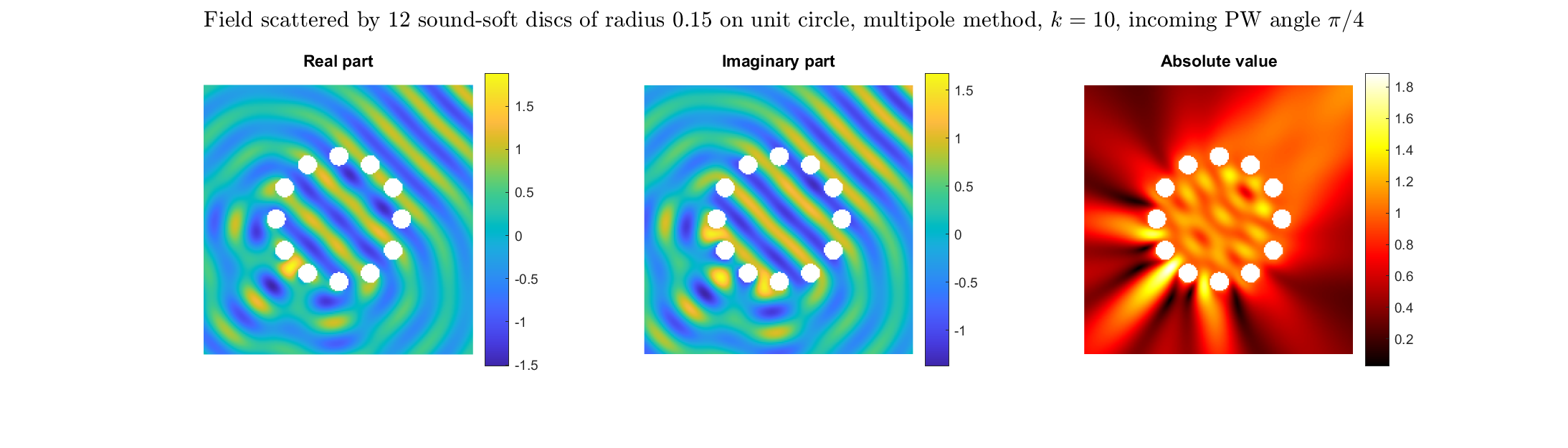
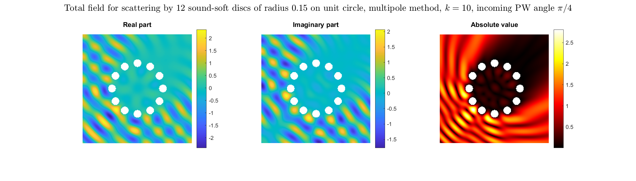
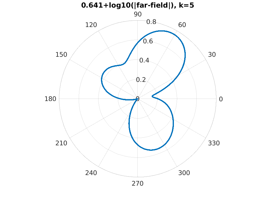
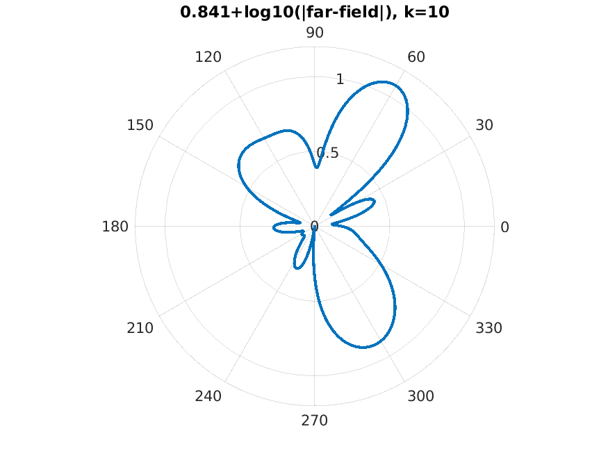
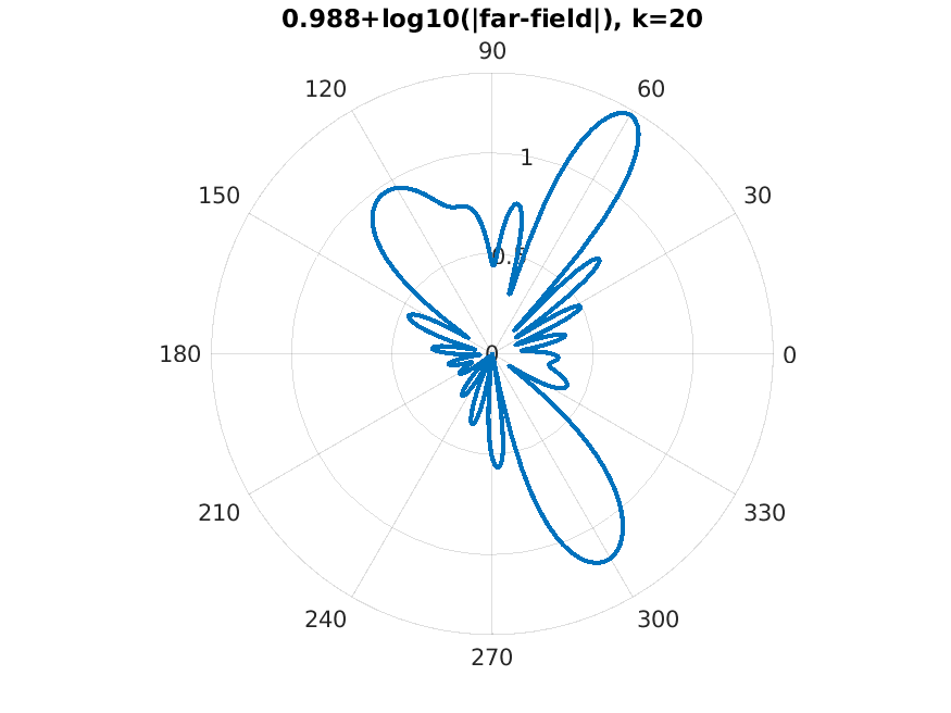
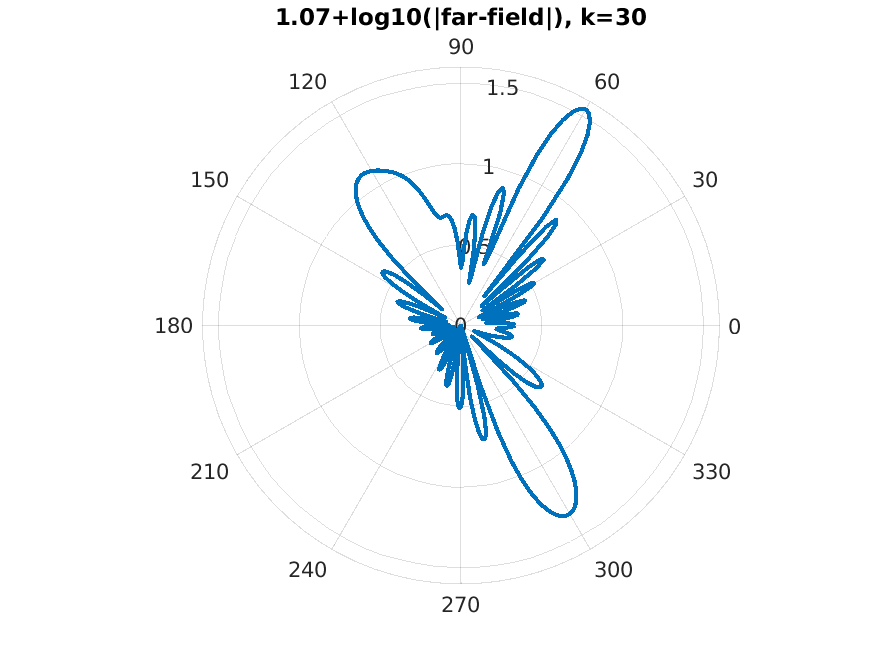
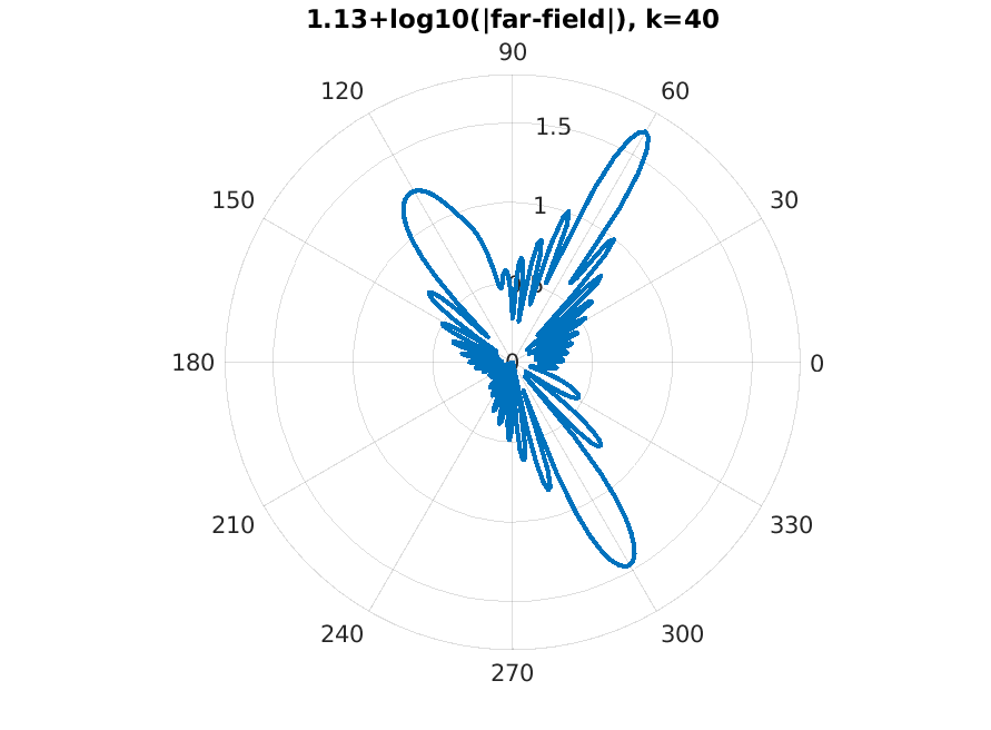
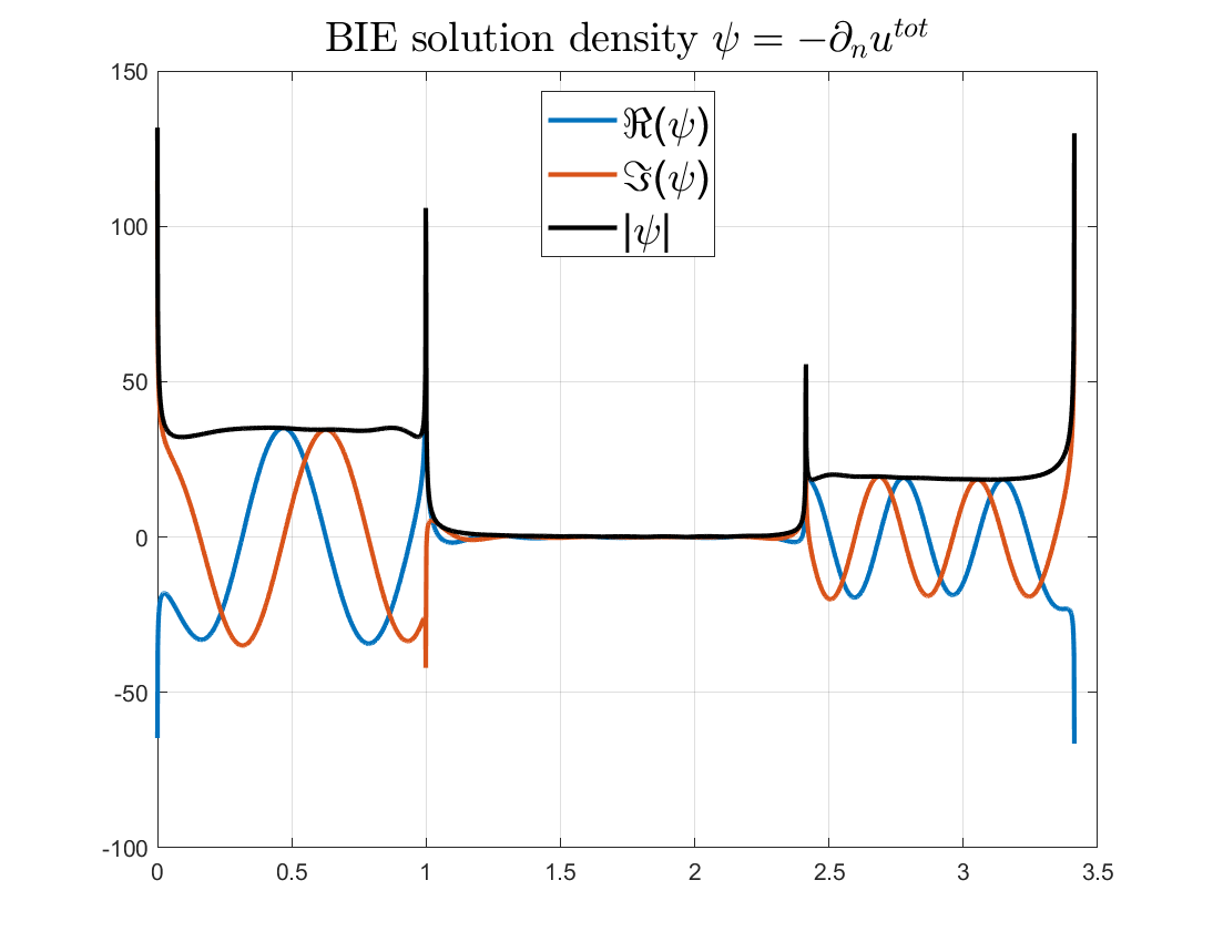
Examples of BEM computations: scattering of a plane wave of direction \((\frac12,\frac{\sqrt3}2)\) by sound-soft polygons.
Triangle with vertices \((0,0),(1,0),(0,1)\), wavenumber \(k=20\).
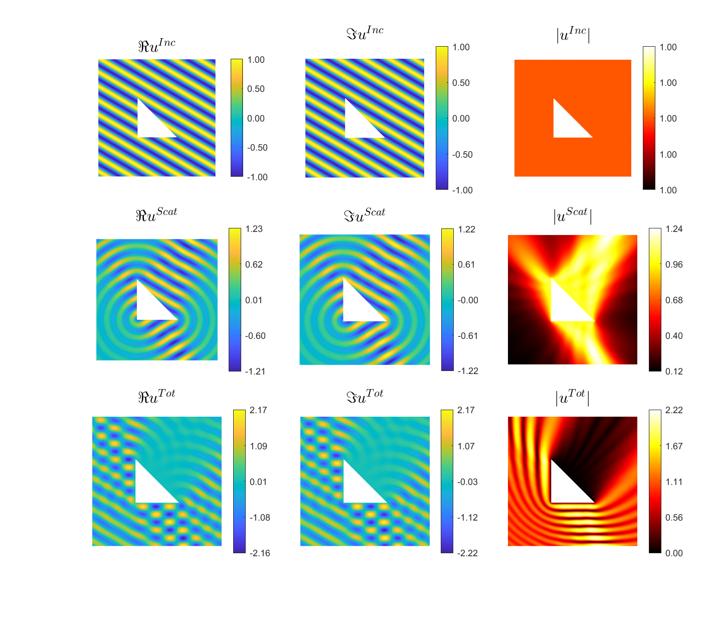 |
Scattered field:
Total field: 
|
|
 |
 | |
 |
Scattered field:
Total field: 
|
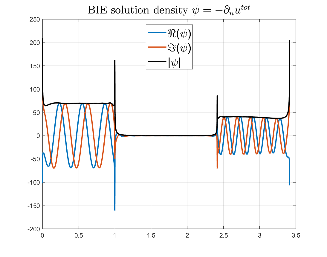
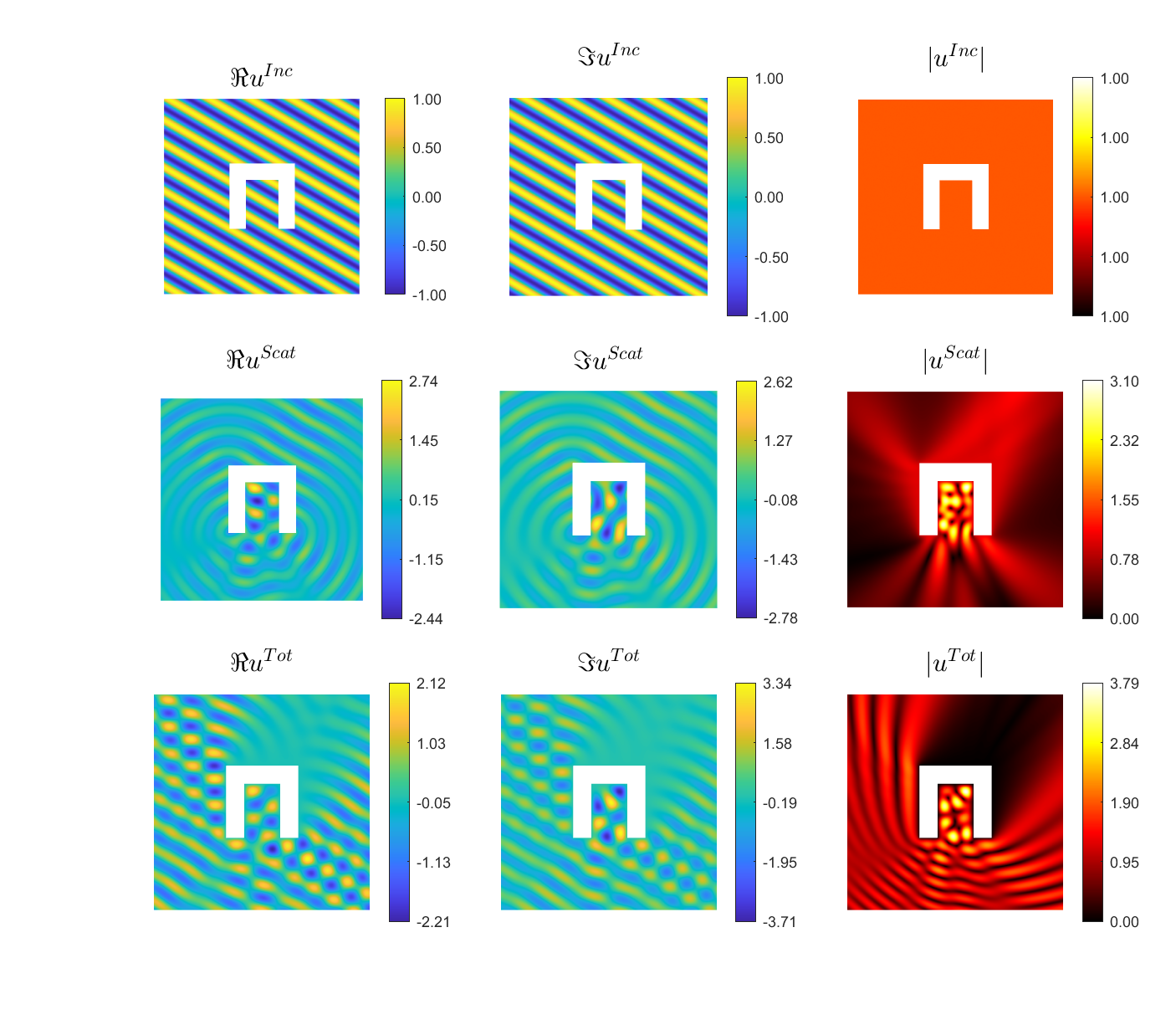
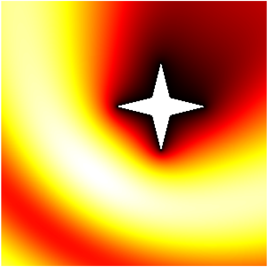
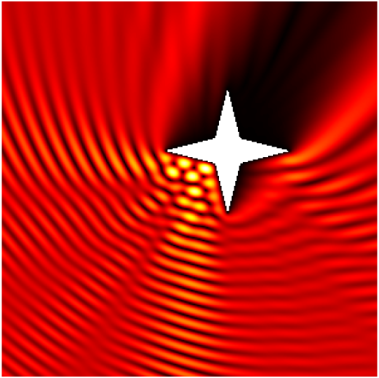
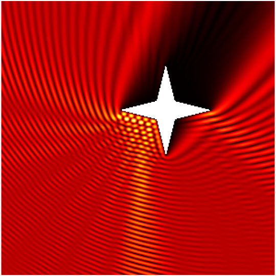
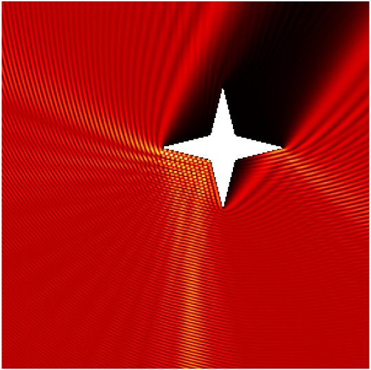
Scattering of a Herglotz function \(u^{Inc}(\mathbf{x})= \int_{\frac\pi4-\frac1{10}}^{\frac\pi4+\frac1{10}}e^{ik((x_1-0.7)\cos\varphi+x_2\sin\varphi)}d\varphi\) by \((0,1.5)^2\setminus(0,1.4]^2\) by a 2D corner reflector, with \(k=70\), plotted on \((-1,2)^2\).
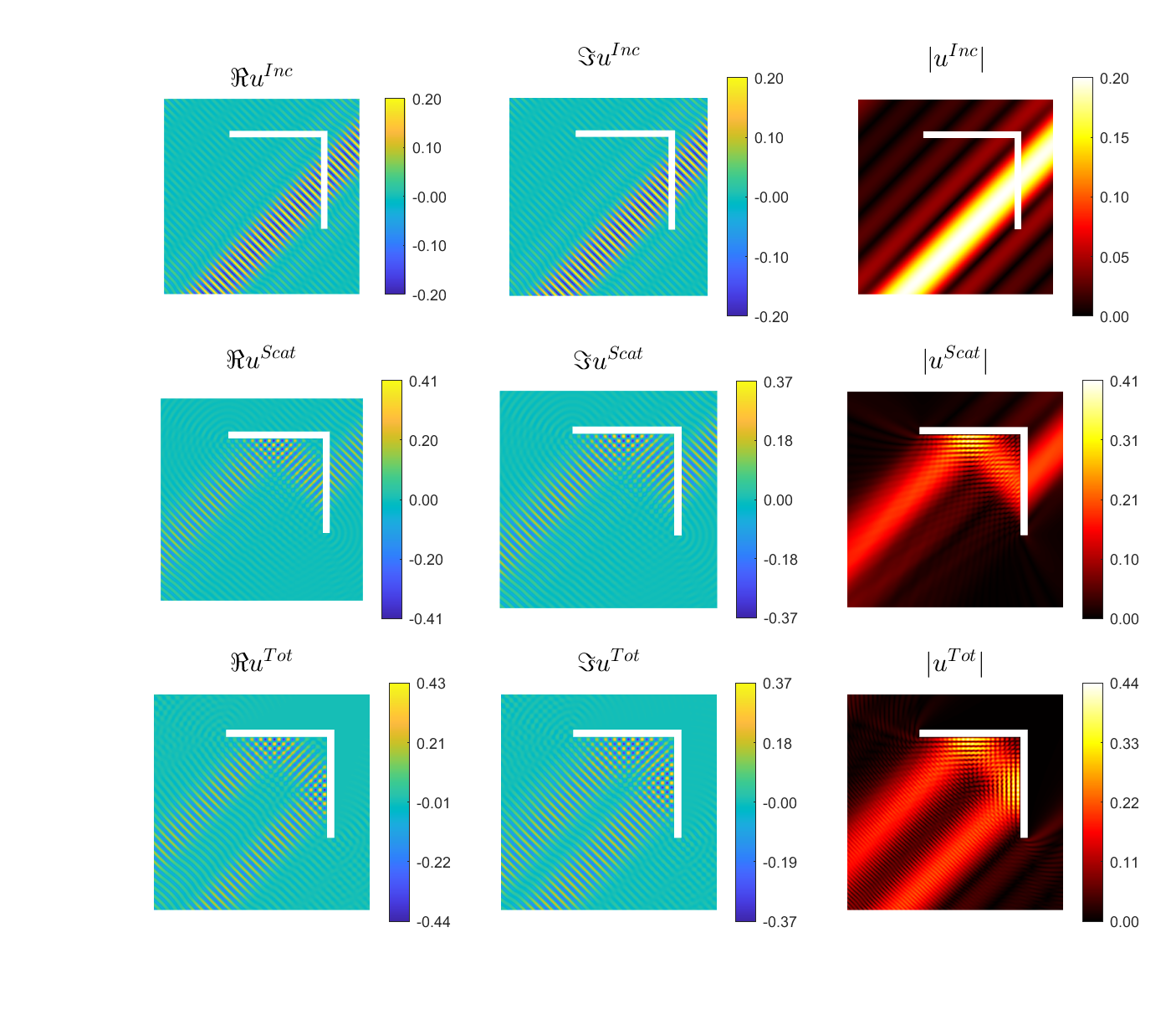 |
Scattered field:
Total field: 
|
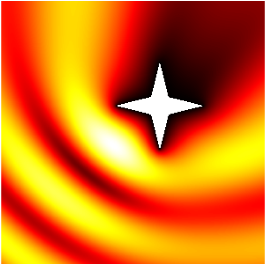
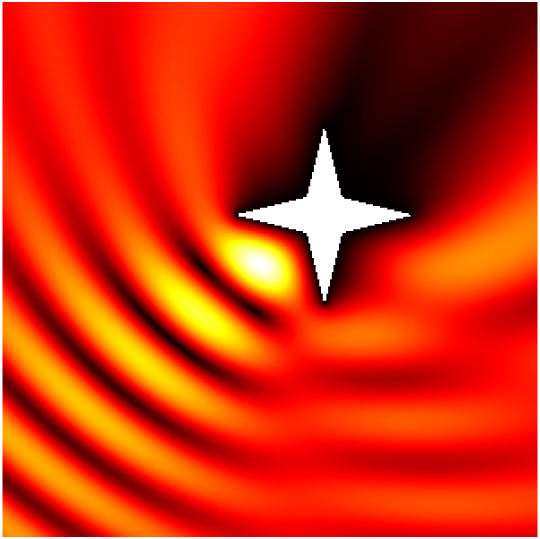
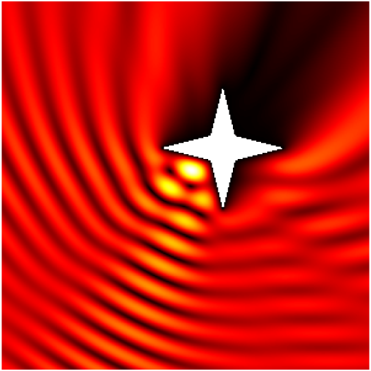
Scattering by the same non-convex obstacle of plane waves with direction \((\frac12,\frac{\sqrt3}2)\) and wavenumbers \(k=1,2,4,8,16,32,64,128\) (total field magnitude).
Babinet principle: scattering by a sound-soft flat screen and diffraction by a sound-hard aperture.
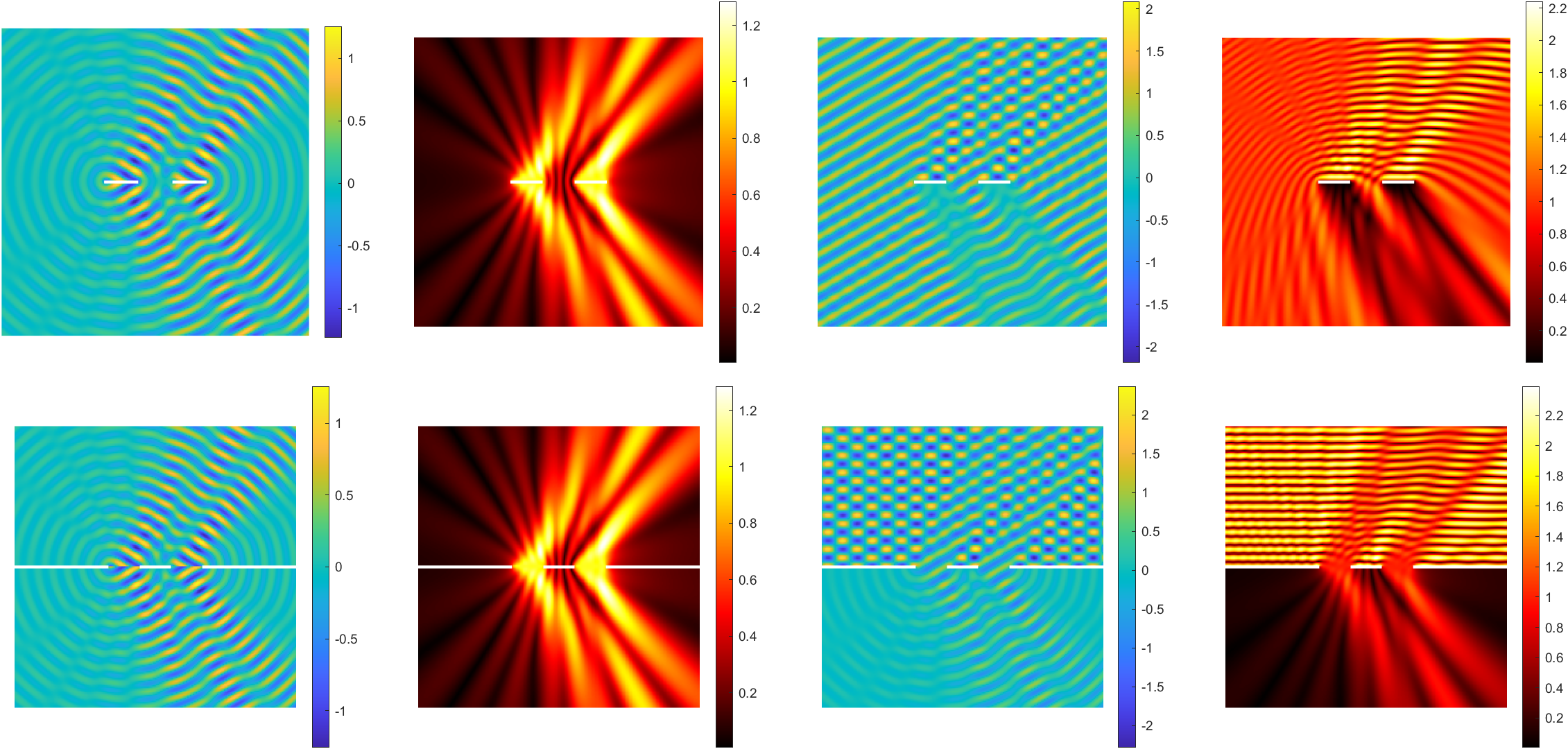
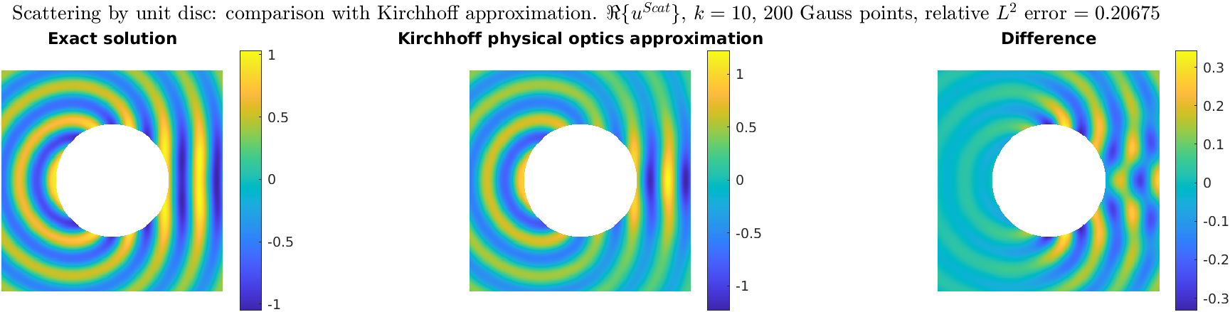
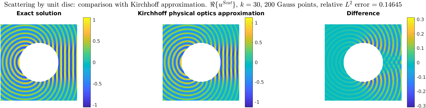
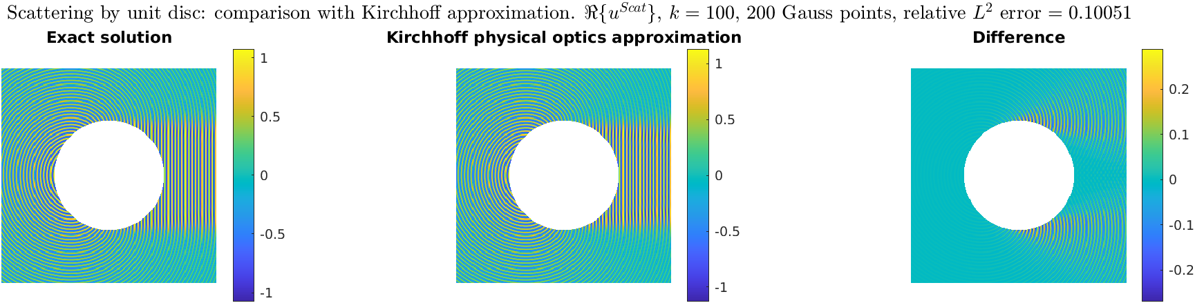
Comparison between SSSP solution and Kirchhoff/physical-optics approximation
Back to the "Advanced numerical methods for PDEs" page.
The Matlab file used to generate most of the figures and the animations (excluding those computed with the BEM):
MNAPDEdrawwaves.m
Benchmark to test the results of the BEM code: file .mat (computed with MPSpack).
Plenty of animations of 2D solutions of the wave equation, interpreted as dimensional reduction of the Maxwell equations, can be found on Robin Hogan's page:
http://www.met.reading.ac.uk/clouds/maxwell/
Other animations of acoustic and elastic waves can be found on the page of Daniel A. Russell:
https://www.acs.psu.edu/drussell/demos.html
A simple interactive introduction to sound propagation is on the page of Bartosz Ciechanowski:
https://ciechanow.ski/sound/